Featured Topics
Featured Products
Events
S&P Global Offerings
Featured Topics
Featured Products
Events
S&P Global Offerings
Featured Topics
Featured Products
Events
S&P Global Offerings
Featured Topics
Featured Products
Events
Language
Featured Products
Ratings & Benchmarks
By Topic
Market Insights
About S&P Global
Corporate Responsibility
Culture & Engagement
Featured Products
Ratings & Benchmarks
By Topic
Market Insights
About S&P Global
Corporate Responsibility
Culture & Engagement

Published: October 1, 2019
Highlights
The way we think about monetary policy has changed with the adoption of quantitative easing (QE): It has moved from being a one-dimensional problem of only setting the policy rate (PR) to a two-dimensional problem of jointly determining the PR and QE.
This new reality requires a framework by the central bank to derive the optimal combination of these two variables given a desired monetary policy stance needed to achieve its policy objective.
Moving to a two-dimensional world for monetary policy raises a host of issues, including the policy rate space (away from zero), the use of dot plots (which represent PR only) to communicate future policy intent, and the predictive power of the yield curve.
This new framework raises the question of whether QE will be permanent, or not, and calls into question the notion that QE cannot begin until the PR reaches the zero bound.
For a PDF of this report, please download.
As we continue to exit the long shadow of the global financial crisis, questions remain about unconventional monetary policies. This will affect the U.S. Federal Reserve first, with other major central banks (eventually) following. Specifically, what will the terminal balance sheet look like? Will central banks go back to using the policy rate (PR) as the only tool with no quantitative easing (QE) and no excess bank reserves (1)? Or will QE--and larger balance sheets--be a permanent fixture of the landscape? How will central banks make that decision?
The Fed's precrisis balance sheet had liabilities consisting of cash in circulation and a small amount of bank reserves needed for the smooth functioning of the interbank market (2). There were no excess reserves. The central bank supplied only the amount of reserves necessary to achieve its target federal funds rate, which was the sole instrument used by the central bank to achieve its policy objectives (3). The size of the balance sheet was around $900 billion (see table 1).
The Fed's maximum post-crisis balance-sheet size reached about $4.5 trillion. How did this quintupling of the balance sheet happen? After hitting the zero bound for its PR in late 2008, and still needing to ease its monetary stance further to achieve its policy objectives, the Fed began to purchase high-quality assets from the market (Treasuries and mortgaged-backed securities). This policy of quantitative easing continued for several rounds, ultimately generating around $2.5 trillion of excess reserves in the banking system (see table 1).
The normalization phase began in December 2015 when the Fed raised its PR from zero, and continued with 25 basis point (bps) increments to the current range of 2.25%-2.50%. Over the same period, a steady reduction in asset holdings began to shrink the balance sheet to around $3.8 trillion at the end of April 2019, with around $1.5 trillion of excess reserves.

With the current debate centered on whether the Fed is approaching--or has reached--the neutral PR, the issue of the terminal balance sheet comes into play. Does the Fed return to its precrisis model of no QE and no excess reserves? This would take the balance sheet down to around $2 trillion, reflecting the demand for cash and the minimum level of bank reserves. Or would some QE remain?
The terminal structure of the central bank balance sheet has clear implications for the number of monetary policy instruments. If we return to the precrisis model, then the PR will be the only instrument the central bank uses to achieve its policy objective. But if QE is a permanent part of the central banking landscape, then there are two instruments: the PR and the amount of QE. In this case, monetary policy needs to determine the PR and the amount of QE jointly to achieve its policy objective. In fact, we would argue that, beginning in December 2015 when the Fed lifted the PR off zero at the same time as having non-zero QE, we had already entered that two-dimensional world, albeit in a very roundabout way.
Launching QE From The Corner: Into The Two-Dimensional Breach
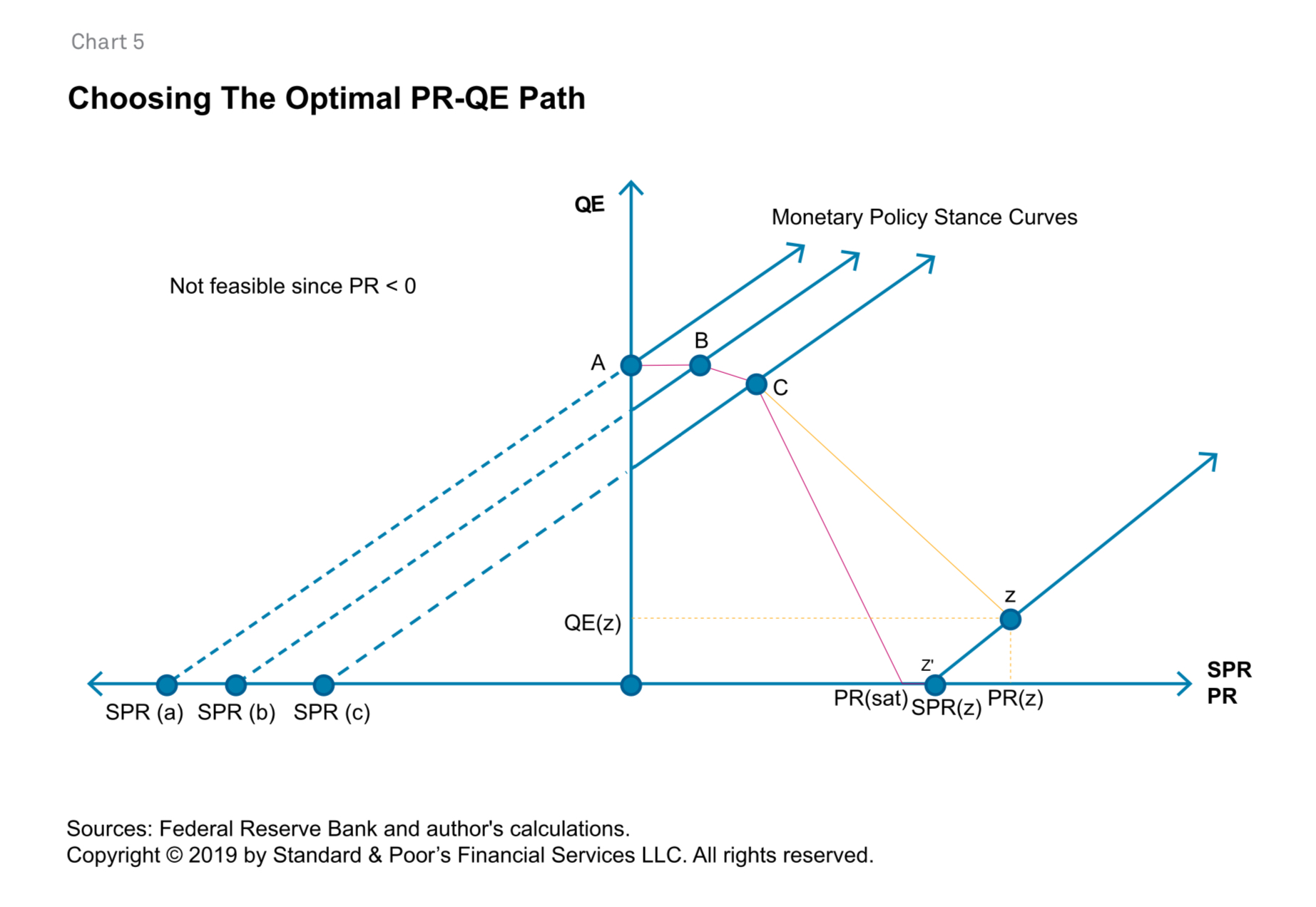
To begin thinking about two-dimensional central bank policy rate space, we can trace the path of U.S. monetary policy over the current rate cycle (see chart 1). The path starts with the precrisis federal funds rate peak of 5.25% in August 2007 (point A). As the crisis intensified, the economy slowed sharply and inflation (expectations) fell, and a much easier monetary policy stance was required. The central bank reduced the federal funds rate quickly, taking the rate left along the PR axis. Given the severity of the crisis and the need for the Fed to ease the policy stance repeatedly, the fed funds rate reached zero in December 2008 (point B).
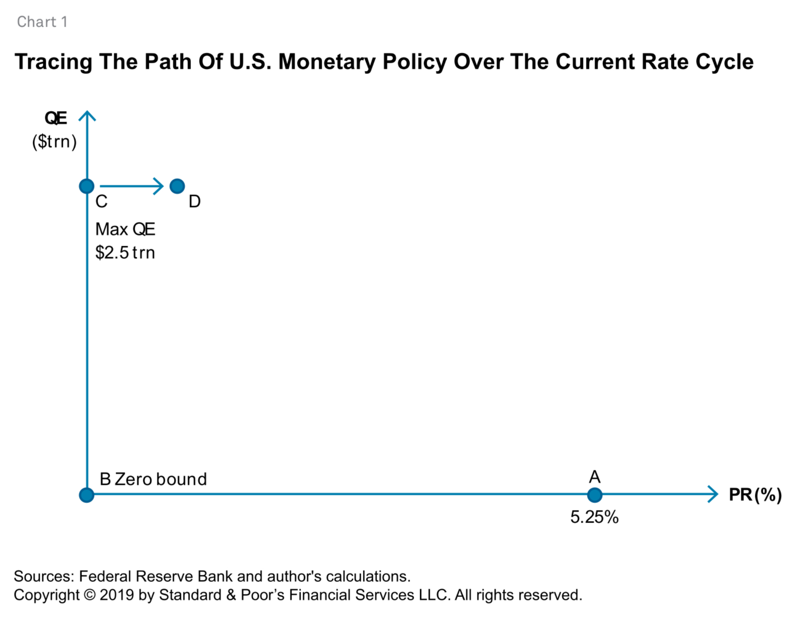
Although the Fed reached the zero (lower) bound for its PR in December 2008, further easing of the monetary policy stance was still required (4). Since PR cuts were no longer feasible, the Fed launched its asset-purchase program in an effort to continue to ease the monetary policy stance. Seven years and three rounds of QE took the Fed to a balance sheet of around $4.5 trillion by December 2015 and excess reserves of around $2.5 trillion (point C). The combination of a zero fed funds rate and maximum level of QE corresponded to the loosest monetary policy stance in the current cycle. From this point on, the issue became the path toward monetary policy normalization.
Importantly, the Fed did not retrace its steps. While the peak-to-trough path in PR-QE space was along points A-B-C, the first move toward policy normalization was to raise the fed funds rate to a range of 25 bps to 50 bps in December 2015 (point C to point D). This was not a retracing of the policy-easing path. In contrast, it represented the first time that the PR and the level of QE were simultaneously both not zero. That is, for the first time, Fed policy entered the interior of the two-dimensional PR-QE space. Previously, the path of PR and QE was a "corner solution" with one or both variables being equal to zero. Now, the policy pair (PR, QE) was in the interior, implying potential trade-offs in choosing the combination of these variables.
The selection of the "interior solution" for the PR and QE raises the question: How can we characterize and then study the optimization of the trade-off between the PR and QE? What does an optimal (PR, QE) path look like as the monetary policy stance normalizes? Answers will require two building blocks: a constraint for "producing" the monetary policy stance and preferences across the two variables.
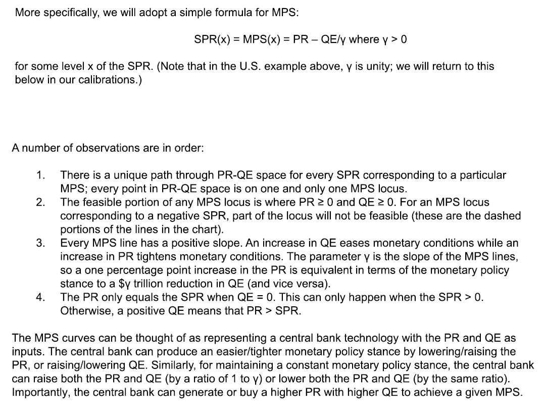
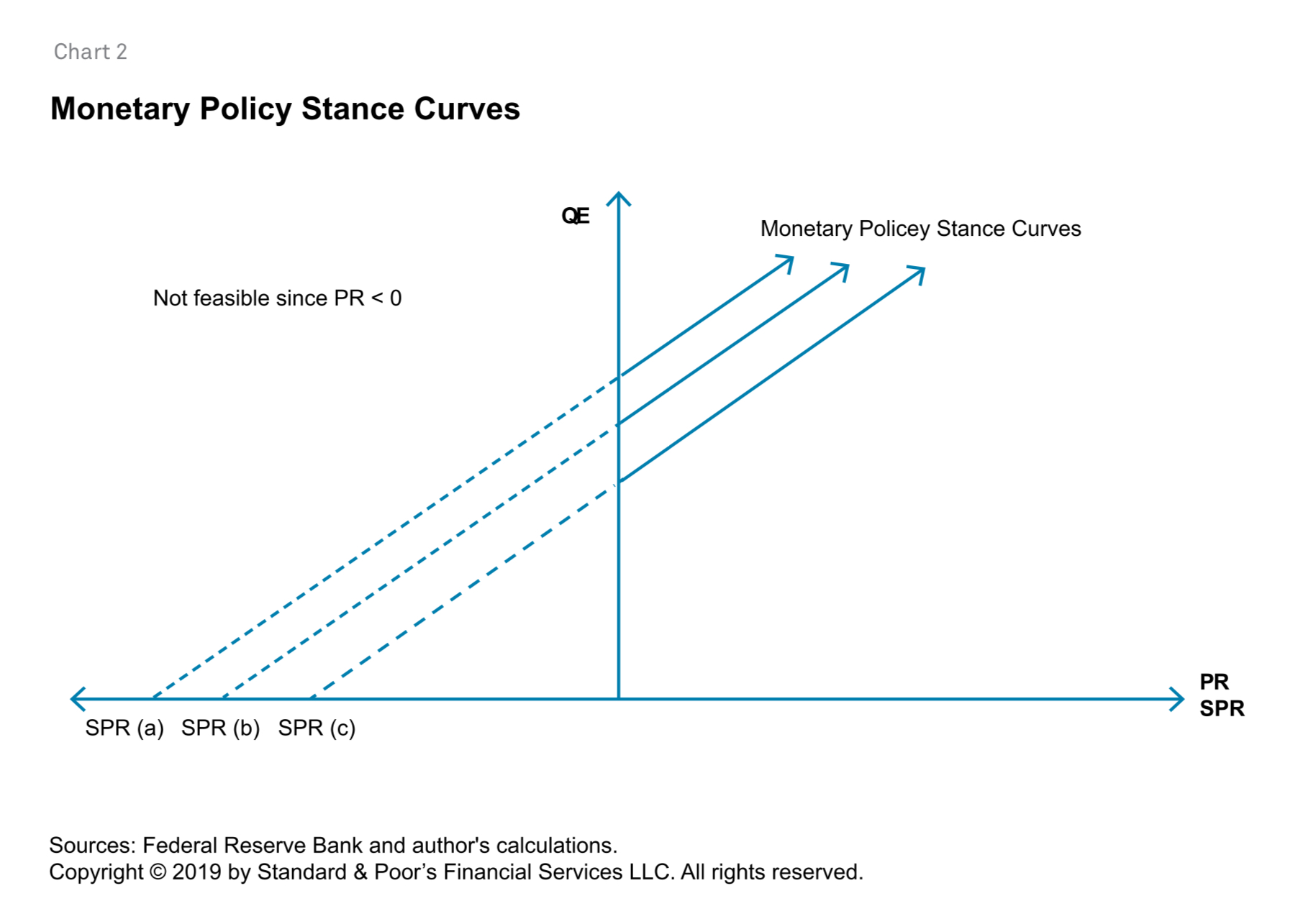
To derive the constraint, we begin with the assertion that any combination of a PR and a level of QE produces a shadow policy rate (SPR). The SPR is the result of mapping the two-variable pair (PR, QE) back to the one-variable world. The twist is that the SPR can take on any value, positive or negative. This is unlike the PR, which can't be negative (5). For example, with the PR at zero, successively higher amounts of QE drove the SPR deeper into negative territory.
How do we generate an SPR? One approach goes through the yield curve (6). For example, in the U.S., $250 billion of asset purchases is estimated to reduce the 10-year term premium by 10 bps. Additionally, the conventional rule of thumb is that a 0.1 percentage point reduction in the 10-year yield is equivalent to a 0.25 percentage point cut in the federal funds rate (7). Thus, each $250 billion in asset purchases would be equivalent to a fed funds rate cut of 0.25 percentage point, and the maximum QE level of around $2.5 trillion would correspond to an SPR of -2.50%.
We can now conclude that a PR-QE pair and its corresponding SPR represent the same monetary policy stance (MPS). Taking this one step further, once we have an SPR for any PR-QE pair, it is straightforward to imagine an entire collection, or "locus," of points that have the same MPS or, equivalently, map to the same SPR. Graphically, this involves connecting the dots through the two points. This locus does not have to be a straight line, but we assume that it is linear for analytical tractability.
Preferences: Central Bank Payoffs
Given a monetary policy stance needed to achieve its target, how will a central bank chose among its PR and QE options in order to maximize their effect?
We will assume that the central bank's payoff function has the following form:
U(PR) + V(QE)
where U is a positive term from raising PR and V is a negative term from raising QE.
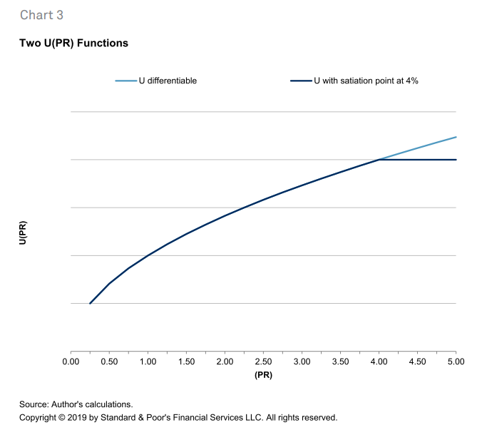
U is the payoff from increasing the PR to provide policy rate space. The idea here is that having policy rate space is valuable, particularly if the PR will need to be cut aggressively in the future to combat a slowdown (8). (This, in turn, implies that the PR is a more effective instrument than QE in such an episode.) Starting from zero, the U function increases quickly, then levels off (9). Importantly, we allow for the possibility of a satiation point for U, meaning there exists a point at which the U function becomes flat and no further payoff is generated by increasing PR further (10) (see chart 3).
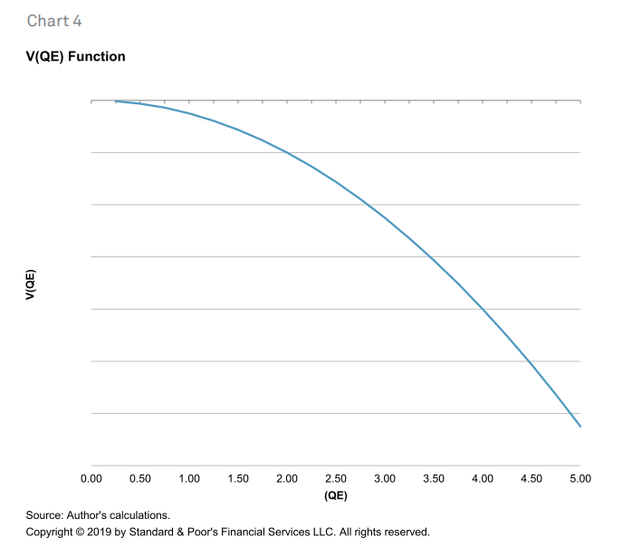
V is the penalty or "disutility" from increasing QE. The idea here is that QE is a distortion to the financial system that lowers rates across the curve and therefore artificially increases asset prices: QE is therefore unambiguously bad (11). This happens through lower discount rates as well as lower borrowing rates. There may also be political economy costs since QE involves paying interest on the excess reserves held by commercial banks (12). These distortive effects of QE are assumed to be increasing as QE rises, so at the margin QE becomes more and more costly (13) (see chart 4).
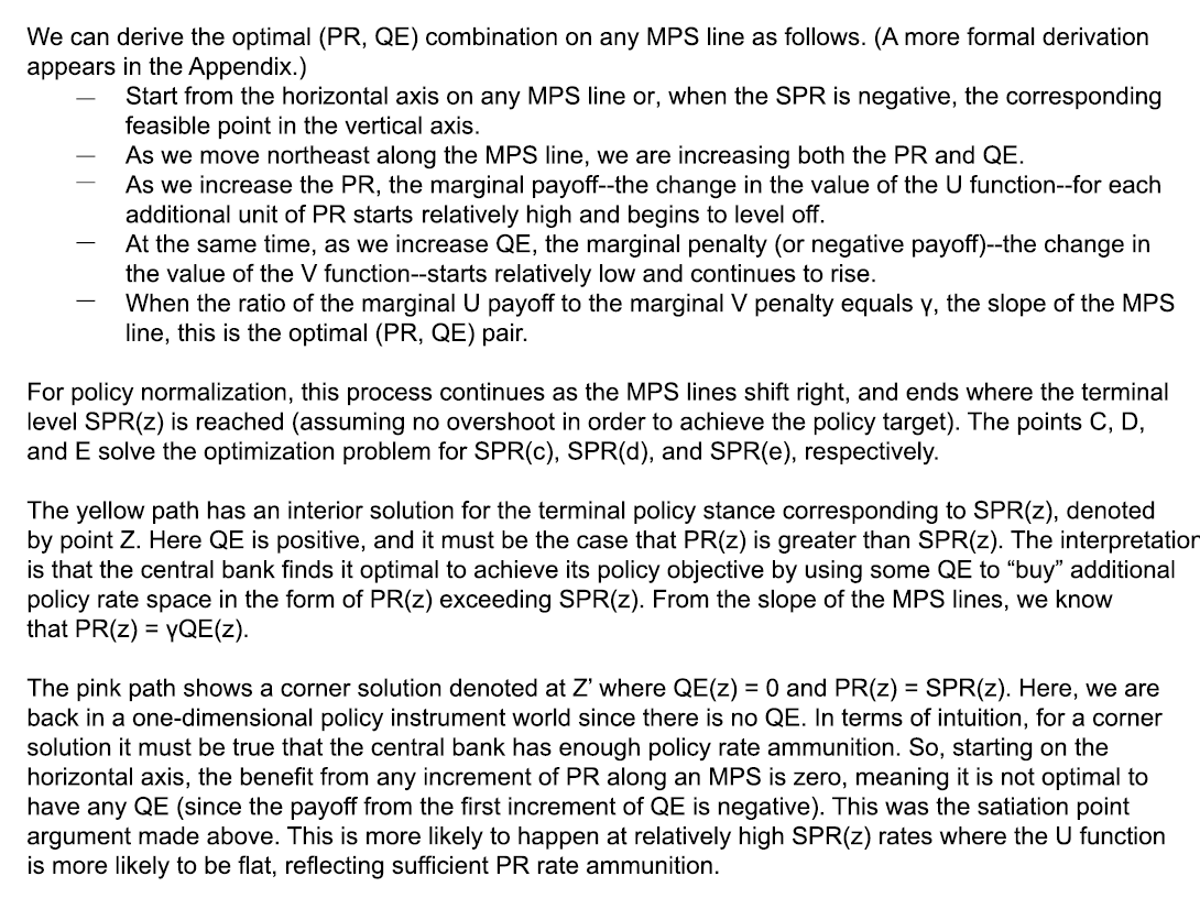
The central bank's payoff function is based on the assumption that initial amounts of PR--and the policy rate space they create--are highly valuable. Central banks will therefore optimally raise the PR at low values, even if it means carrying a relatively large amount of QE. However, as the benefit of policy rate space wanes, additional units of the PR become less valuable, so it is less optimal to carry a large amount of QE. As the MPS lines continue to shift to the right, and the monetary policy stance normalizes, the interplay between the value of more policy rate space and the cost of QE will determine where the central bank ends up in PR-QE space.
With policy stance production constraints and a payoff function in hand, we can now derive the central bank's optimal PR-QE path. We can also investigate the "terminal" value of QE to see whether it is positive, or not.
The central bank's optimization problem is as follows: Once the SPR needed to achieve the policy objective has been selected, choose the (PR, QE) pair along the corresponding MPS line that maximizes U(PR) + V(QE). Do this each time as the required SPR and MPS line changes. The process ends when we reach the neutral or terminal SPR* (see chart 5).
A Calibrated Solution
If we determine a specific, "closed form" solution, this will allow us to add some numbers and calibrate the model so that we can see how it operates in a recognizable range of variables. The calibration is based on U.S. variables and should be taken as a rough approximation.
To keep things as simple as possible, we assume that:
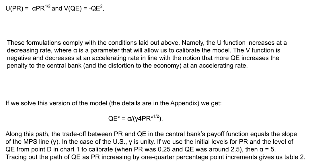


So when the fed funds rate is 5% (10%), the optimal amount of QE is about $0.5 trillion ($0.4 trillion).
Finally, the issue of the "terminal" point for the monetary policy cycle is problematic because we don't know whether the terminal point is in terms of the PR (for example, using the Fed's dot plots) or the SPR/monetary policy stance. Using the PR, the calibrated model suggests that QE should be around $0.75 trillion when the fed funds rate is between 2.75% and 3.00%, the "long run" dot plot.
This analysis raises a number of issues.
To address these issues definitively, more work is needed to refine and stress test the model. The trade-off between the PR and QE in achieving a given MPS is unlikely to be linear; that assumption was made for analytical convenience. The separable payoff function of the central bank was also adopted for convenience, and the robustness of the results with respect to different formulations of that function will need to be ensured as well. Nonetheless, we will likely be in a two-dimensional monetary policy world for the foreseeable future. The issue becomes how to think about formulating and executing optimal monetary policy in that world for central banks to achieve their objectives.


